pyFRET Tutorial
Installing pyFRET
- pyFRET is available as a module on PyPI, the Python Packagae Index.
If you are already familiar with python and PyPI:
- make sure you have numpy, scipy, matplotlib and scikit learn installed
- pip install pyFRET
If you are completely new to python, there are three stages to getting pyFRET up and running:
- Getting Python
- Getting Anaconda (extra packages for scientific computing)
- Getting scikit learn
- Getting pyFRET
Instructions for all three steps follow:
Getting Python
If you are not already using python for programming, you may need to install python. Here are some instructions:
These pages also provide useful links to tutorials for programming in python.
Please note: pyFRET was written using python 2. The latest release of python 2 is python 2.7.6. The pyFRET library is also compatible with python 3, for which the latest release is python 3.4.
Getting Anaconda
Once you have python up and running, you need to make sure you have all the packages that pyFRET needs to work properly. Specifically, you will need:
- scipy
- numpy
- matplotlib
- scikit learn
If you have used python for scientific programming before, you may already have these installed. If so, you are ready to install pyFRET.
If you haven’t used python much, you will need to get these packages. The easiest way is to download Anaconda, which will install 125 python packages used for scientific programming.
Some hints for installing Anaconda:
- Their instructions are very clear and easy to follow
- During the installation, you will be asked if you want to add the anaconda binary directory to your PATH environment variable. Say yes. This means that every time you use python, you will have acces to all the packages installed by Anaconda.
Getting Scikit learn
Scikit learn is not installed by default with Anaconda. However, once you have Anaconda installed, it is easy to install scikit learn. From the Anaconda terminal, type:
$ conda install scikit-learn
If you are not using Anaconda and you need to install scikit learn, there are comprehensive instructions on the scikit-learn website.
Getting pyFRET
Now you are ready to install pyFRET.
Open a terminal window and type:
$ pip install pyFRET
Installing pyFRET using pip will automatically detect whether you have the required packages and will install them for you at the same time as pyFRET is installed. Sadly, scipy and matplotlib don’t install very nicely using pip install, so this will make a big mess.
If you need to install these packages, get them before you try downloading pyFRET. Scipy has dependencies on numpy, so you will need to install numpy first.
The best instructions for getting all of the required packages can be found on the Scipy installation page.
Using pyFRET
To use pyFRET to analyse your data, you must first import the module into your python program. You can use:
import pyfret
This will import the whole module. However, it is easier to import pyFRET and pyALEX separately:
from pyfret import pyFRET as pft
from pyfret import pyALEX as pyx
This will let you use their functions directly.
Sample code that uses pyFRET to analyse smFRET data can be found in ALEX_example.py and FRET_example.py. These programs use configuration files to load parameters for the analysis. These configuration files are ALEX_config.cfg and FRET_config.cfg. These files can be found in the /bin folder of the pyFRET download.
To provide further illustration of how pyFRET can be used, below are some examples of things that you can do using pyFRET.
Using pyFRET.pyFRET
Now that you have pyFRET imported into your program, you are ready to use it to analyse data. Let’s start with a simple analysis of some FRET data.
First, you need to initialize a FRET data object to hold your data.
If you have a list of .csv files (here called file1, file2 and file3), you can do this:
my_directory = "path/to/my/files"
list_of_files = ["file1.csv", "file2.csv", "file3.csv"]
my_data = pft.parse_csv(my_directory, list_of_files)
This will store your data as two arrays of values, named donor and acceptor, in an object called my data. You can print these arrays like this:
print my_data.donor
print my_data.acceptor
Similarly, if you have a list of binary files with a .dat extension, like those used in the Klenerman group, you can do this:
my_directory = "path/to/my/files"
list_of_files = ["file1.dat", "file2.dat", "file3.dat"]
my_data = pft.parse_bin(my_directory, list_of_files)
A handy hint about files: A dataset typically consists of many files in the same directory, with the same base name but different file numbers. To quickly build a list of files to be parsed by one of these function, you can do something like this:
# The info you need
my_directory = "path/to/my/files"
no_files = 20       # how many files you have
files = []          # empty list to hold file names
name = "mydata"     # main part of file name
filetype = "dat"    # file extension

# Making your list of files
for n in range(no_files):
    # for n = 1, full_name = mydata0001.dat
    full_name = ".".join(["%s%04d" %(name, i), filetype])
    files.append(full_name)

# Reading your data
FRET_data = pft.parse_bin(my_directory, files)
Now you are ready to start manipulating the data.
To subtract background autofluorescence:
auto_donor = 0.5 # donor autofluorescence
auto_acceptor = 0.3 # acceptor autofluorescence
my_data.subtract_bckd(auto_donor, auto_acceptor)
To select bursts using AND thresholding:
threshold_donor = 20 # donor threshold
threshold_acceptor = 20 # acceptor threshold
my_data.threshold_AND(threshold_donor, threshold_acceptor)
To select bursts using SUM thresholding:
threshold = 30 # threshold
my_data.threshold_SUM(threshold)
To remove cross-talk from bursts:
cross_DtoA = 0.05 # fractional crosstalk from donor to acceptor
cross_AtoD = 0.01 # fractional crosstalk from acceptor to donor
my_data.subtract_crosstalk(cross_DtoA, cross_AtoD)
To calculate the FRET proximity ratio of bursts, you can use the proximity_ratio function:
gamma = 0.95 # instrumental gamma factor (default value 1.0)
E = my_data.proximity_ratio(gamma=0.95)
You can also build FRET histogram directly from the donor and acceptor data. To make a FRET histogram, use the function build_histogram, which will calculate the proximity ratio internally. This function has several optional additions.
The simplest option is just to make a histogram, and save the frequencies and bin centres in a .csv file:
filepath = "path/to/save/histogram"
csvname = my_histogram
g_factor = 0.95 # instrumental gamma factor
my_data.build_histogram(filepath, csvname, gamma=g_factor, bin_min=0.0, bin_max=1.0, bin_width=0.02)
You can also save an image of the histogram:
filepath = "path/to/save/histogram"
csvname = my_histogram
g_factor = 0.95 # instrumental gamma factor
my_data.build_histogram(filepath, csvname, gamma=g_factor, bin_min=0.0, bin_max=1.0, bin_width=0.02, \
image = True, imgname = my_histogram, imgtype="png")
Finally, you can fit the histogram with one or more gaussian distributions and save the parameters of the fit in a csv file. This will also make an image of the histogram overlaid with the gauss fit.
filepath = "path/to/save/histogram"
csvname = my_histogram
g_factor = 0.95 # instrumental gamma factor
n_gauss = 2     # number of gaussians to fit
my_data.build_histogram(filepath, csvname, gamma=g_factor, bin_min=0.0, bin_max=1.0, bin_width=0.02, \
image=True, imgname=my_histogram, imgtype="png", gauss=True, gaussname="gaussfit", n_gauss=n_gauss)
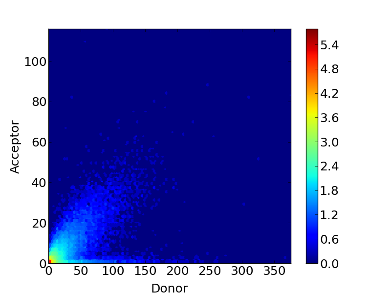
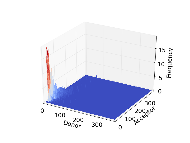
As well as making histograms, you can also make some other plots to display your data. For example, a heatmap or 3D plot of event frequencies:
# make a heatmap
filepath = "path/to/save/image"
plotname = my_plot
my_data.make_hex_plot(filepath, plotname, imgtype="pdf", binning="log")

# make a 3D plot
filepath = "path/to/save/image"
plotname = my_3d_plot
my_data.make_3d_plot(filepath, plotname, imgtype="pdf")
This makes images like these:
For more information on the pyFRET library, more functions and more detail, please see the reference:
Using pyFRET.pyALEX
pyALEX is for data collected using alternating laser excitation. Many of the functions are similar to those used in pyFRET. Here is a quick oveview.
First, you need to initialize an ALEX data object to hold your data.
If you have a list of .csv files (here called file1, file2 and file3), you can do this:
my_directory = "path/to/my/files"
list_of_files = ["file1.csv", "file2.csv", "file3.csv"]
my_data = pft.parse_csv(my_directory, list_of_files)
This will store your data as four arrays of values (see below) in an object called my_data. The four data channels in an ALEX experiment are:
- D_D: Donor channel when the donor laser is on
- D_A: Donor channel when the acceptor laser is on
- A_D: Acceptor channel when the donor laser is on
- A_A: Acceptor channel when the acceptor laser is on
You can print these arrays like this:
print my_data.D_D
print my_data.D_A
print my_data.A_D
print my_data.A_A
Similarly, if you have a list of binary files with a .dat extension, like those used in the Klenerman group, you can do this:
my_directory = "path/to/my/files"
list_of_files = ["file1.dat", "file2.dat", "file3.dat"]
my_data = pft.parse_bin(my_directory, list_of_files)
A handy hint about files: A dataset typically consists of many files in the same directory, with the same base name but different file numbers. To quickly build a list of files to be parsed by one of these function, you can do something like this:
# The info you need
my_directory = "path/to/my/files"
no_files = 20       # how many files you have
files = []          # empty list to hold file names
name = "mydata"     # main part of file name
filetype = "dat"    # file extension

# Making your list of files
for n in range(no_files):
    # for n = 1, full_name = mydata0001.dat
    full_name = ".".join(["%s%04d" %(name, i), filetype])
    files.append(full_name)

# Reading your data
FRET_data = pft.parse_bin(my_directory, files)
Now you are ready to start manipulating the data.
To subtract background autofluorescence:
autoD_D = 0.5 # donor autofluorescence (donor laser)
autoD_A = 0.3 # donor autofluorescence (acceptor laser)
autoA_D = 0.5 # acceptor autofluorescence (donor laser)
autoA_A = 0.8 # acceptor autofluorescence (acceptor laser)
my_data.subtract_bckd(auto_donor, auto_acceptor)
To subtract leakage and direct excitation from the FRET channel:
l = 0.05 # fractional leakage from donor excitation into acceptor channel
d = 0.03 # fractional contribution of direct acceptor excitation by donor laser
my_data.subtract_crosstalk(l, d)
The key innovation of ALEX is to select events based on their photon stoichiometry – the fraction of all observed photons that were emitted by the acceptor dye.
Both the Proximity Ratio, E, and the stoichiometry, S, can be calculated explicitly:
    g_factor = 0.95 # the gamma factor
E = my_data.proximity_ratio(gamma=g_factor) # Proximity ratio
S = my_data.stoichiometry(gamma=g_factor) # Stoichiometry
Then you can remove singly-labelled molecules that give events with extreme stoichiometries:
S = my_data.stoichiometry(gamma=g_factor)
    S_min = 0.2 # minimum S
S_max = 0.8 # maximium S
S = my_data.stoichiometry_selectiony(S, S_min, S_max)
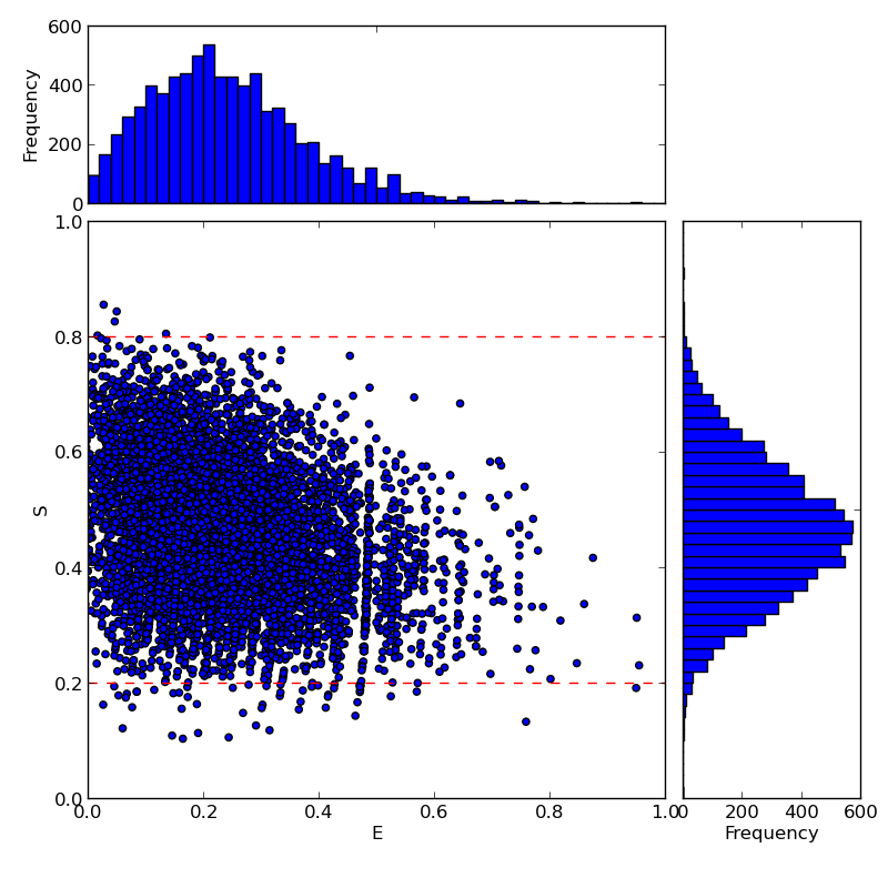
However, E and S can also be calculated in a single step, combined with burst selection based on S, using the scatter_hist function. This will also plot and optionally save a scatter plot of your data, with projections of E and S:
g_factor = 0.95 # the gamma factor
S_min = 0.2
S_max = 0.8
filepath = "path\to\my\file"
filename = "scatter_plot"
scatter_hist(self, S_min, S_max, gamma=1.0, save=True, filepath=filepath, imgname=filename, imgtype="png")
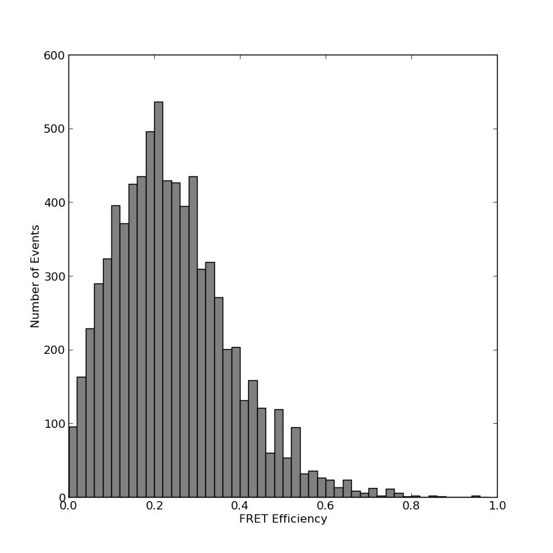
You can also make a separate histogram of the selected events. The histogram frequencies and bin centres will be saved in a csv file. You can also optionally save an image of the histogram and fit it to one or more gaussian distributions.
g_factor = 0.95 # the gamma factor
S_min = 0.2
S_max = 0.8
filepath = "path\to\my\file"
filename = "E_histogram"
img = "E_plot"
build_histogram(filepath, filename, gamma=1.0, bin_min=0.0, bin_max=1.0, bin_width=0.02, image = True, imgname = img, imgtype="png")
The scatterplot and FRET Efficency histograms look like this:
For more details about pyALEX, please see the detailed documentation:
Using The Burst Search Algorithms
pyFRET now includes burst search algorithms for both FRET and ALEX data.
The algorithms implemented are the All Photons Burst Search (APBS) AND Dual Channel Burst Search (DCBS) algorithms described in Nir et al.’s 2006 paper.
To use these algorithms, you will need time-binned data that has been binned on a timescale much shorter than the typical dwell time of a molecule in the confocal volume. A suitable bin-time would be 0.01 ms for freely diffusing molecules, although shorter bin times can also be used.
These burst search algorithms identify fluorescent bursts by grouping together photons that reach the photon counting devices within some short time window of each other. According to Nir et al:
The start (respectively, the end) of a potential burst is detected when the number of photons in the averaging window of duration T is larger (respectively, smaller) than the minimum number of photons M.
A potential burst is retained if the number of photons it contains is larger than a minimum number L.
In the APBS method, photons from all channels are summed to give a total number of photons which is then evaluated in each window. In the DCBS method, photons encountered during donor exciation periods are considered separately from those encountered during acceptor excitation periods. To be accepted as a burst, both donor and acceptor dyes must be active throughout the entire burst.
To use the burst search algorithms in pyFRET, it is necessary to first initialize a pyFRET data object. The burst search algorithm can then be used:
# The info you need
my_directory = "path/to/my/files"
no_files = 20       # how many files you have
files = []          # empty list to hold file names
name = "mydata"     # main part of file name
filetype = "dat"    # file extension

# Making your list of files
for n in range(no_files):
    # for n = 1, full_name = mydata0001.dat
    full_name = ".".join(["%s%04d" %(name, n), filetype])
    files.append(full_name)

# Reading your data
FRET_data = pft.parse_bin(my_directory, files)

# calling APBS algorithm
T1 = 50             # time window (bins)
L1 = 50             # first threshold
M1 = 30             # second threshold

bursts_APBS = FRET_data.APBS(T1, L1, M1)

# calling DCBS algorithm
T2 = 50             # time window (bins)
L2 = 25             # first threshold
M2 = 15             # second threshold

bursts_DCBS = FRET_data.APBS(T2, L2, M2)
According to Nir et al., appropriate values for the APBS algorithm are:
- T = 0.5 ms
- L = 50
- M = 30
Similarly for the DCBS algorithm:
- T = 0.5 ms
- L = 25
- M = 15
The value of T used in the pyFRET burst search algorithm depends on the bin-time used. If a 0.01 ms bin-time is used, then to achieve a window size of T = 0.5 ms, a value of T = 50 bins should be used in calling the burst search algorithm.
The burst search algorithm returns a FRET_bursts data object, which can be used in the same way as the original FRET data object. However, an additional denoise_bursts function is provided, which will denoise identified bursts in a manner proportional to the burst duration. Crosstalk subtraction is unchanged.
# subtract background
N_D = 0.005   # donor noise per bin
N_A = 0.004   # acceptor noise per bin
bursts_APBS.denoise_bursts(N_D, N_A)

cross_DtoA = 0.05 # fractional crosstalk from donor to acceptor
cross_AtoD = 0.01 # fractional crosstalk from acceptor to donor
bursts_APBS.subtract_crosstalk(cross_DtoA, cross_AtoD)

# plot FRET histogram
filepath = "path/to/save/histogram"
csvname = "my_histogram"
g_factor = 0.95 # instrumental gamma factor
bursts_APBS.build_histogram(filepath, csvname, gamma=g_factor, bin_min=0.0, bin_max=1.0, bin_width=0.02)
The FRET_bursts data object has three extra attributes, burst_starts, burst_ends and burst_len, which are arrays of (respectively) the start time, end time and duration (in time bins) of each identified burst. The FRET_bursts object also has an additional plotting function, that can be used to display the relationship between burst duration and brightness:
# the burst_len attribute
print bursts_APBS.burst_len

# plotting the relationship between burst duration and brightness
filepath = "path/to/save/plot"
imgname = "my_plot"
bursts_APBS.scatter_intensity(filepath, imgname, imgtype="pdf")
Similarly for ALEX data:
# The info you need
my_directory = "path/to/my/files"
no_files = 20       # how many files you have
files = []          # empty list to hold file names
name = "mydata"     # main part of file name
filetype = "dat"    # file extension

# Making your list of files
for n in range(no_files):
    # for n = 1, full_name = mydata0001.dat
    full_name = ".".join(["%s%04d" %(name, n), filetype])
    files.append(full_name)

# Reading your data
ALEX_data = pyx.parse_bin(my_directory, files)

# calling APBS algorithm
T1 = 50             # time window (bins)
L1 = 50             # first threshold
M1 = 30             # second threshold

bursts_APBS = ALEX_data.APBS(T1, L1, M1)

# calling DCBS algorithm
T2 = 50             # time window (bins)
L2 = 25             # first threshold
M2 = 15             # second threshold

bursts_DCBS = ALEX_data.APBS(T2, L2, M2)

# make scatterhist plot with projections
S_min = 0.2
S_max = 0.8
filepath = "path/to/save/plot"
ALEX_data.scatter_hist(S_min, S_max, gamma=1.0, save=True, filepath=filepath, imgname="scatterhist", imgtype="png")
RASP: Recurrence Analysis of Single Particles
Finally, the FRET_bursts data can be analysed using the Recurrence Analysis of Single Particles (RASP) method described by Hoffmann et al. (Phys Chem Chem Phys. 2011 13(5):1857-1871). Fluorescent bursts that occur within a short time interval of each other have a high probability of having been generated by the same fluorescent molecule reentering the confocal volume. RASP can be used to identify bursts that occurred within a short time period of bursts with a specified FRET efficiency.
From Hoffmann et al,:
First, the bursts b2 must be detected during a time interval between t1 and t2 (the ‘recurrence interval’, T = (t1,t2)) after a previous burst b1 (the ‘initial burst’). Second, the initial bursts must yield a transfer efficiency, E(b1), within a defined range, Delta E1 (the ‘initial E range’).
In pyFRET’s implementation of RASP, t1 and t2 are named Tmin and Tmax. The initial E range is given by Emin and Emax:
# initial E range: 0.4 < E < 0.6
Emin = 0.4
Emax = 0.6

# Time interval for re-occurrence
# given in number of bins
Tmin = 1000
Tmax = 10000

# selcting re-ocurring bursts
recurrent_bursts = bursts_APBS.RASP(Emin, Emax, Tmin, Tmax)

# histogram of re-occurring bursts
recurrent_bursts.build_histogram(filepath, csvname, gamma=g_factor)
The Sample Data
Included in /bin is some sample data that you can use to check that your installation of pyFRET is working correctly.
To reproduce our data analysis, from the /bin folder in pyFRET, type:
$ python FRET_example.py 10bp_FRET_config.cfg
This will execute the program FRET_example.py using the parameters stored in the configuration file 10bp_FRET_config.cfg, to analyse smFRET data from dual labelled DNA duplex, with a 10 base-pair separation between the dye attachment sites. There are four more smFRET datasets to analyse (4, 6, 8 and 12 bp separations) with similar configuration files.
Similarly, you can reproduce our analysis of the equivalent ALEX data using:
$ python ALEX_example.py 10bp_ALEX_config.cfg
There is also some sample data and a sample script for burst search in FRET data:
$ python FRET_bursts_example.py FRET_bursts_config.cfg
Right now, the configuration file parser that is used in ALEX_example.py and FRET_example.py runs only with a python 2.x installation. We are working on making an equivalent set of files for use with python 3.x distributions.
To learn more about how configuration files work and how you can use them to analyse your own data please see the configparser documentation:
You can open both the configuration files and the example python scripts in a text editor (like Sublime or Gedit) to see how the configuration files are used by the python program: